Method #1. Sparklines in Excel
One of the groundbreaking innovations in the last version of Microsoft Excel 2010/2013 is the possibility of using sparklines – minicharts placed within cells and demonstrating the dynamics of numeric data:

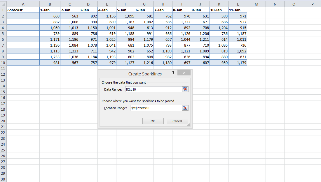
In order to create such minicharts, it is necessary to select those cells, where we want to put it, and then use buttons of Sparklines group from Insert tab:

In the appearing dialogue box, you need to specify the range of source data and the output range:
Created minicharts may be formatted and adjusted in every way by means of Design dynamic tab:

In particular, you can easily change the color of lines and columns of the sparkline and mark minimum and maximum values with special colors:

Since the sparkline basically plays the role of cell background (it is not a separate graphical object), it would not make any problems if you need to enter text, numbers or other information into the cell.
What can you do, if you have an old Excel version at the moment? Or you need such type of chart, which is not offered in the sparklines set? Let’s move forward to the next method!
Method 2. Extra add-ons for microcharts
Actually, the idea of such charts was in the air for quite a while. Even for Excel 2003, there were several add-ons with similar functionality, the most known of them were the remarkable add-on Sparklines (free) by Edward Tufte, and BonaVista microcharts (paid) and Bissantz SparkMaker (paid). The only drawback is that add-ons must be installed on all computers, where you are planning to work with a file containing such charts.
Method 3. N-times iteration of symbols
The “budget choice” for one-dimensional microcharts is repeating similar symbols for imitation of a bar chart. For this purpose, you may use text function REPT, which can iteratively output any selected symbol into the box. In order to output irregular symbols (knowing their code), you may use CHAR function. Essentially, it looks like this:

A symbol with code 103 is a black rectangular from Webdings font, so don’t forget to set this font for boxes C2:C12. Also, you can play with symbols from other fonts, for example, a symbol with code 110 from Wingbinds font was used in E column.
Method 4. Macros
This method is an improved version of previous method, where a set of repeating symbols (“I” symbol is used) is created not by a formula, but a simple user-defined function on VBA. At that, a separate column is created for each box, since the function uses line break symbol after each number. It looks like this:

In order to use this trick in your file, you’ll need to open VBA editor (Alt+F11), add a new module to the book (Insert -> Module) and copy Nanochart function code into the module:
                    Function NanoChart(rng As Range) As String
                        Const MaxSymbols = 10

                        For Each cell In rng
                            outstr = outstr & WorksheetFunction.Rept("|", cell / WorksheetFunction.Max(rng) * MaxSymbols) & Chr(10)
                        Next cell
                        NanoChart = outstr
                    End Function
Then, we paste NanoChart function into the needed cells indicating numeric data as arguments (as shown on the picture above). It is necessary to enable word wrap and 90 degrees turn (Format -> Cells -> Alignment) for the resulting cells with microcharts. MaxSymbols constant sets a length of the highest column in the minihistogram.
One more method was fairly seen at http://www.dailydoseofexcel.com/. It involves addition of user-defined VBA function for automatic construction of sparklines (tiny charts within cells) to the file. Open VBA editor (Alt+F11), add a new module to the book (Insert -> Module) and copy this Visual Basic code into the module:
                    Function LineChart(Points As Range, Color As Long) As String
                        Const cMargin = 2
                        Dim rng As Range, arr() As Variant, i As Long, j As Long, k As Long
                        Dim dblMin As Double, dblMax As Double, shp As Shape

                        Set rng = Application.Caller

                        ShapeDelete rng

                        For i = 1 To Points.Count
                            If j = 0 Then
                                j = i
                            ElseIf Points(, j) > Points(, i) Then
                                j = i
                            End If
                            If k = 0 Then
                                k = i
                            ElseIf Points(, k) < Points(, i) Then
                                k = i
                            End If
                        Next
                        dblMin = Points(, j)
                        dblMax = Points(, k)

                        With rng.Worksheet.Shapes
                            For i = 0 To Points.Count - 2
                                Set shp = .AddLine( _
                                    cMargin + rng.Left + (i * (rng.Width - (cMargin * 2)) / (Points.Count - 1)), _
                                    cMargin + rng.Top + (dblMax - Points(, i + 1)) * (rng.Height - (cMargin * 2)) / (dblMax - dblMin), _
                                    cMargin + rng.Left + ((i + 1) * (rng.Width - (cMargin * 2)) / (Points.Count - 1)), _
                                    cMargin + rng.Top + (dblMax - Points(, i + 2)) * (rng.Height - (cMargin * 2)) / (dblMax - dblMin))

                                On Error Resume Next
                                j = 0: j = UBound(arr) + 1
                                On Error GoTo 0
                                ReDim Preserve arr(j)
                                arr(j) = shp.Name
                            Next

                            With rng.Worksheet.Shapes.Range(arr)
                                .Group

                                If Color > 0 Then .Line.ForeColor.RGB = Color Else .Line.ForeColor.SchemeColor = -Color
                            End With

                        End With

                        LineChart = ""
                    End Function

                    Sub ShapeDelete(rngSelect As Range)
                        Dim rng As Range, shp As Shape, blnDelete As Boolean

                        For Each shp In rngSelect.Worksheet.Shapes
                            blnDelete = False
                            Set rng = Intersect(Range(shp.TopLeftCell, shp.BottomRightCell), rngSelect)
                            If Not rng Is Nothing Then
                                If rng.Address = Range(shp.TopLeftCell, shp.BottomRightCell).Address Then blnDelete = True
                            End If

                            If blnDelete Then shp.Delete
                        Next
                    End Sub
Now, a new function LineChart with two arguments (range and chart color code) has appeared in the User-Defined category of the function master. If you paste it into a blank cell, for example, on the right from the numeric line, and then copy it on the whole column (as usual), you will get quite a nice presentation of numeric data in the form of minicharts:

Original article here